
In the last post, we explored simple linear regression, where one feature predicts one target. That single line already gave us pretty good insights into relationships between variables. But real-world problems don’t just depend on one factor.
Let’s take some examples: House prices are influenced by more than just size. Salary depends on more than just years of experience (even though we did see a pretty good simple linear regression there). When more than one variable contributes to the outcome, we move to multiple linear regression.
Multiple linear regression extends the same principles as before, but with more predictors. The goal remains the same: to find the best-fitting model that describes how the features (x) explain variation in a target variable (y).
The model
The formula for multiple linear regression looks like this: y=β0+β1x1+β2x2+…+βnxn+ε
Where:
- y is the dependent variable (the value we want to predict).
- x₁, x₂, … xₙ are the independent variables (features).
- β₀ is the intercept.
- β₁, β₂, … βₙ are the coefficients that measure how each feature influences y.
- ε is the error term (unexplained variation).
Each coefficient represents the average change in y when that feature changes by one unit, assuming all other features remain constant.
Example in Python
Instead of a tiny artificial dataset, let’s look at a more realistic example.
In the accompanying Kaggle notebook, we use the Ames Housing dataset and build a model to predict house prices using features such as:
- Overall quality
- Living area (square feet)
- Total basement area
- Number of bathrooms
- Garage size
These are features that intuitively relate to property value. Below is a simplified illustration of how we fit the model using scikit-learn:
from sklearn.linear_model import LinearRegression
from sklearn.model_selection import train_test_split

features = [
    "OverallQual",
    "GrLivArea",
    "GarageCars",
    "GarageArea",
    "TotalBsmtSF"
]
X = df[features].fillna(0)
y = df["SalePrice"].fillna(df["SalePrice"].median())

X_train, X_test, y_train, y_test = train_test_split(X, y, test_size=0.2, random_state=42)

model = LinearRegression().fit(X_train, y_train)
r2 = model.score(X_test, y_test)
We then extract the model coefficients and metrics such as R² and adjusted R² in the notebook.
Full notebook:
https://www.kaggle.com/code/alexandermaitken/house-prices-multiple-linear-regression
Interpreting the results
Suppose our model returns the following:
- An intercept of about -$99,000
- Each increase in OverallQual adds roughly $23,600 to the price
- Each additional square foot of living area (GrLivArea) adds about $45
- Each extra garage car space adds around $14,500
- Each additional square foot of basement (TotalBsmtSF) adds about $31
- GarageArea appears to add about $17 per square foot, but it is not statistically significant once GarageCars is included
- The model achieves an R² of 0.76, meaning it explains about 76 percent of the variation in sale price
You could interpret this as: higher-quality homes, larger living spaces, bigger basements, and more garage capacity are all associated with higher sale prices. The effect of garage area becomes negligible once we account for the number of car spaces, which suggests those features overlap. That is a sign of multicollinearity, and in practice you would typically remove or combine one of them.
The negative intercept simply reflects that the model is trying to fit a line in a space where a “zero-sized house with zero features” does not exist. It is not meaningful in this context.
Overall, the model captures a substantial portion of the variation in house prices and aligns with intuition: larger, higher-quality homes with more livable space tend to sell for more.
In practice, looking at summary statistics alone is not enough. A good regression workflow pairs the numbers with diagnostic checks to make sure the model is stable and meaningful.
Multicollinearity
In multiple regression, multicollinearity occurs when features are highly correlated with each other. It can make coefficients unstable and difficult to interpret.
For example, if you include both house size and number of rooms, those two variables may carry similar information. The model will still produce coefficients, but small changes in the data can cause large swings in those numbers.
You can detect multicollinearity using a correlation matrix or by calculating the Variance Inflation Factor (VIF) for each feature. A high VIF (typically above 5 or 10) suggests a problem.
You can also use a pairwise plot to visually inspect the data. Here you look for a straight-line trend or tight clusters, which can indicate collinearity.
In our example, the pairwise plots show that some features move together, like garage size and number of garage spaces, but we do not see points forming a perfect straight line. That means the relationship is there, but not extremely strong. We also checked the Variance Inflation Factor (VIF) to quantify this. A VIF above 5 suggests moderate multicollinearity, and above 10 suggests a strong issue. In our case, the highest VIF value is around 5.5, which tells us there is some overlap between features, but not enough to cause issues. In short, the features are related in a natural way, but not so much that they cause problems for our model.
If features are too correlated, you can:
- Remove one of them.
- Combine them (for example, rooms per square foot).
Feature selection
Feature selection helps you decide which variables to include in your regression model. Including too many features can lead to overfitting, while too few can cause underfitting. There are three main strategies: forward, backward, and stepwise (mixed) selection.
Forward selection
Start with no features and add them one by one.
At each step, the feature that improves the model the most (based on a metric like adjusted R² or AIC) is added.
You stop when adding more features does not meaningfully improve the model.
Backward elimination
Start with all candidate features and remove them one by one.
At each step, the least significant feature (for example, the one with the highest p-value above a threshold like 0.05) is dropped.
You stop when all remaining features are statistically significant.
Stepwise (bidirectional) selection
Combines the two methods.
At each iteration, you can add or remove features based on their contribution to the model’s performance.
This dynamic process continues until no further improvement occurs.
In Python
In our notebook, we use forward and backward feature selection to automatically choose meaningful predictors.
from sklearn.feature_selection import SequentialFeatureSelector
from sklearn.linear_model import LinearRegression

model = LinearRegression()

# Forward selection (start with no features)
sfs_forward = SequentialFeatureSelector(
    model, n_features_to_select=5, direction="forward", scoring="r2"
)

# Backward elimination (start with all features)
sfs_backward = SequentialFeatureSelector(
    model, n_features_to_select=5, direction="backward", scoring="r2"
)
These techniques validate our manual selections and help avoid including redundant or noisy variables.
Full forward/backward example:
https://www.kaggle.com/code/alexandermaitken/house-prices-multiple-linear-regression.
Model evaluation
The same metrics apply as before:
- R² indicates how much variance the model explains.
- Adjusted R² compensates for the number of features. It increases only if a new variable improves the model more than would be expected by chance.
- P-values show whether individual coefficients are statistically significant.
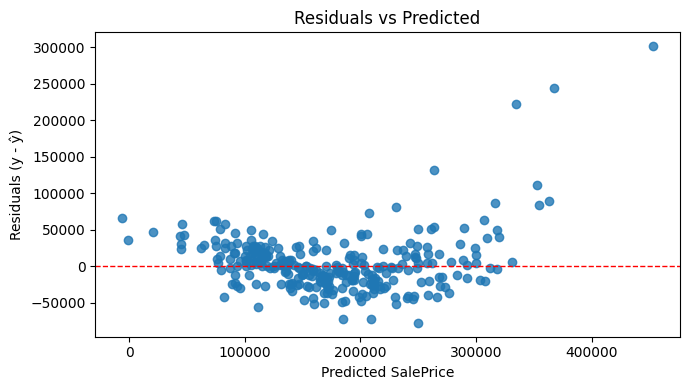
You can also examine residual plots to check whether the assumptions of linearity and constant variance still hold.
Common pitfalls
- Overfitting: Adding too many features can make the model fit noise in the training data rather than true patterns.
- Omitted variable bias: Leaving out important variables can distort the effect of those that remain.
- Interpreting coefficients causally: A relationship does not imply causation. Coefficients show association, not proof of cause and effect.
Being aware of these helps prevent misleading conclusions.
Summary and what’s next
Multiple linear regression lets us handle more realistic problems where several factors interact. It builds directly on the ideas from simple regression and introduces new concepts like multicollinearity and adjusted R².
Before we move into regularisation and non-linear models, there is one more important branch of regression to explore: logistic regression. While multiple linear regression predicts continuous values like price, logistic regression helps us predict categories, such as whether a house is above or below a price threshold, or whether a customer is likely to churn.
We will explore logistic regression in the next part of this series.
Leave a Reply