
When I first thought about machine learning, it seemed like a scary topic. Coming from product engineering, I often heard about models, black boxes, and mysterious choices around which model to use. It felt inaccessible and mathematical.
Recently, I decided to go beyond that assumption. To my surprise, a lot of it builds on concepts I had already seen in my MBA statistics class. The simplest place to start is simple linear regression, which turns out to be one of the best gateways into machine learning.
Understanding linear regression is not just about drawing a line through data. It is about understanding how models learn relationships, estimate parameters, and make predictions. These same ideas underpin far more advanced algorithms, from neural networks to gradient boosting.
Supervised learning
The type of problem that linear regression solves belongs to a class called supervised machine learning. In supervised learning, we provide the model with data that already has labels. The model learns to predict a target (output) based on one or more features (inputs).
Other forms of machine learning, like unsupervised learning, do not use labels. Instead, they look for patterns in the data by themselves. For now, we will stay within the supervised world.
The linear regression model
At its core, linear regression looks for a straight-line relationship between an input variable x and an output variable y:
y = β0 + β1x + ε
Where:
- y is the dependent variable (response or target).
- x is the independent variable (predictor or feature).
- β₀ is the intercept (the value of y when x is 0).
- β₁ is the slope of the line (how much y changes for every one-unit change in x).
- ε is the error term (the difference between the predicted and actual values).
The goal of the model is to find the line that best fits the data. The most common approach is the least squares method, which finds the line that minimises the sum of the squared residuals. A residual is simply the difference between what the model predicts and what is actually observed.
A simple example in Python
Here is how that looks in practice using the scikit-learn library. We will use the Salary dataset on Kaggle. You can run the example in my Kaggle notebook and follow along: dataset • notebook.
# Simple Linear Regression with residuals - Salary Dataset
# --------------------------------------------------------
# Dataset: https://www.kaggle.com/datasets/abhishek14398/salary-dataset-simple-linear-regression
# Requirements: pandas, matplotlib, scikit-learn, numpy

import matplotlib.pyplot as plt
from sklearn.linear_model import LinearRegression
from sklearn.metrics import mean_squared_error, r2_score

# ----- 1) Load data -----
df = pd.read_csv("/kaggle/input/salary-dataset-simple-linear-regression/Salary_dataset.csv")
print(df.head())

# ----- 2) Fit model -----
X = df[["YearsExperience"]].values
y = df["Salary"].values

model = LinearRegression()
model.fit(X, y)

y_pred = model.predict(X)
residuals = y - y_pred

# Model stats
intercept = model.intercept_
slope = model.coef_[0]
r2 = r2_score(y, y_pred)
rmse = np.sqrt(mean_squared_error(y, y_pred))

print(f"Intercept (β0): {intercept:.2f}")
print(f"Slope (β1):     {slope:.2f}")
print(f"R²:             {r2:.3f}")
print(f"RMSE:           {rmse:.2f}")
The intercept represents β₀, the slope represents β₁, and the R² value tells us how well the model explains the variance in the data. An R² close to 1 means the model fits the data well.
Intercept (β0): 24848.20
Slope (β1):     9449.96
R²:             0.957
RMSE:           5592.04
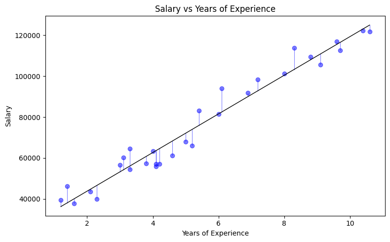
If you plot this dataset as a scatterplot and draw the fitted line, you will see how the model approximates the trend. Visualising this is a great way to build intuition about how models capture patterns in data.
plt.figure(figsize=(8, 5))
plt.scatter(df["YearsExperience"], df["Salary"], label="Observed", alpha=0.8)
plt.plot(df["YearsExperience"], y_pred, color="red", label="Best fit line", linewidth=2)
Evaluating the model
When you fit a linear regression model, statistical tools will often return metrics like the p-value, confidence interval, and R².
- P-value: Tests whether there is a meaningful relationship between x and y. A small value (typically < 0.05) suggests the relationship is statistically significant.
- Confidence interval: Gives a range where the true value of the slope is likely to fall, usually with 95% confidence.
- R² value: Shows how much of the variation in y is explained by x. Higher is better, but values too close to 1 can signal overfitting.
- RMSE (Root Mean Squared Error): Measures the average prediction error in the same units as the target variable. Smaller values indicate that predictions are closer to actual results.
These metrics help us interpret how meaningful the relationship is. But they are only part of the story.
Checking assumptions and residuals
Linear regression relies on a few important assumptions:
- Linearity – The relationship between x and y is linear.
- Independence – The residuals (errors) are independent of each other.
- Constant variance – The residuals have constant variance across all levels of x (homoscedasticity).
- Normality – The residuals are roughly normally distributed.
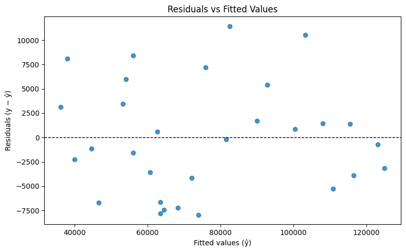
After fitting a model, it is good practice to plot the residuals. If they form a random pattern around zero, your model assumptions likely hold. If there are patterns or the variance increases with x, the model may not be the right fit.
Choosing your features
Even in simple regression, you might wonder how to choose which features to use. A correlation matrix is a good starting point. It shows how strongly each variable relates to the others. Highly correlated features can cause multicollinearity, which distorts regression results when you move to multiple regression (for our dataset in Kaggle, we don’t need to do this as we only have two features).
A pair plot can help visualise these relationships. Each scatterplot in the grid shows how two variables interact, while the diagonal plots show the distribution of individual variables. Hot spots in a correlation matrix or strong diagonal patterns in a pair plot can help you see where relationships are strongest.
Summary and what’s next
Simple linear regression is the first step toward understanding how machines learn from data. It introduces the key concepts of features, targets, parameters, and error. These ideas are the foundation of more advanced methods.
Next, I will explore multiple linear regression, where we move from a single feature to several. This brings new challenges, such as correlated features, overfitting, and diminishing returns on additional predictors.
Understanding these basics will make everything that follows in machine learning feel far less mysterious.
Leave a Reply